
Poisson Processes and Data Loss
C. Traylor
There are many applications for counting arrivals over time. Perhaps I want to count the arrivals into a store, or shipments into a postal distribution center, or node failures in a cloud cluster, or hard drive failures in a traditional storage array. It's rare that these events come neatly, one after the other, with a constant amount of time between each event or arrival. Typically those interarrival times,the time between two events in a sequence arriving, are random. How then do we study these processes?
Poisson Process
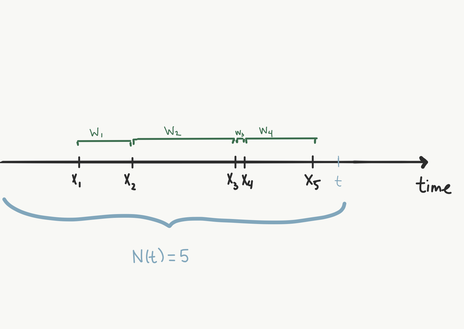 Here, the axis shows time passing. Each X is the occurrence of an event, and the W's denote the time between event arrivals. If we're currently at the point in time of the blue t, 5 events have occurred. Notice that the times of occurrence are random. If we started this process over again, we wouldn't necessarily have 5 events occurring by the time we hit that blue t again.
The Poisson process is acounting process, under the assumption that events arrive randomly according to certain rules. A counting process, denoted ${N(t)}$, is simply a random process where $N(t)$ is the total number of events that have occurred up to some time t. There are a few other defining characteristics that make a counting process a Poisson process:
Here, the axis shows time passing. Each X is the occurrence of an event, and the W's denote the time between event arrivals. If we're currently at the point in time of the blue t, 5 events have occurred. Notice that the times of occurrence are random. If we started this process over again, we wouldn't necessarily have 5 events occurring by the time we hit that blue t again.
The Poisson process is acounting process, under the assumption that events arrive randomly according to certain rules. A counting process, denoted ${N(t)}$, is simply a random process where $N(t)$ is the total number of events that have occurred up to some time t. There are a few other defining characteristics that make a counting process a Poisson process:
(1) $N(0) = 0$
This just covers us mathematically. We can't have a negative number of events, and at time 0, we start with no events.
(2) $\{N(t), t \geq 0\}$ hasindependent increments.
What do we mean by independent increments? Suppose we have two time intervals, measured from time $t=0$: $I_{1} = [1,4]$ and $I_{2} = [5,7]$. Then the number of arrivals that occurred during $I_{1}$, which we will call $N(4-1)$ and is a random variable, must be independent of the random variable $N(7-5)$, the number of arrivals that happened in time interval $I_{2}$
Of course, I picked specific numbers, and just two intervals, but this has to be true for all disjoint intervals of time and of any size. In other words, for $0 \leq t_{1} < t_{2} < \ldots < t_{n} < \infty$, $N(t_{2} - t_{1})$,$N(t_{3} - t_{2})$, all the way to$N(t_{n} - t_{n-1})$ must be independent random variables, no matter how big $n$ gets, or the size of the intervals.
(3) $\{N(t), t \geq 0\}$ has stationary increments
Let's take an interval of time of a fixed length, say 2. So the interval $[1,3]$, or $[103,105]$. Those two intervals are the same length, but occur at different points in time. If a random process has stationary increments, the probability distribution for the number of events occurring in $[1,3]$ is the same as that for the number of events occurring in $[103,105]$. The probability distribution of the number of events that occur in all intervals of the same length is the same. We write this as $N(t_{2}+s) - N(t_{1} + s) \sim^{\mathcal{D}} N(t_{2}) - N(t_{1})$ for any two points in time $t_{1}, t_{2}$ and any positive shift $ s > 0$. s = 101 in our numeric example. This is important, because now we can characterize what that probability distribution is:
(4)The number of events in any interval of length $t$ has a Poisson distribution with mean $\lambda t$
This means that we have anaverage arrival rate of $\lambda$ events per unit time, and the probability that $n$ events occur in a time interval of length $t$, regardless of where that interval is (written $P(N(t+s)-N(t))$), can be given by the Poisson distribution with pdf
$$P(N(t+s)-N(t) = n) = e^{-\lambda t}\frac{(\lambda t)^{n}}{n!}$$
For example, if, on average, 5 people come into a grocery store per hour, then $\lambda = 5$ and the probability that there will be 10 arrivals in the next hour is
$$P(N(t+1)-N(t) = 10) = e^{-5\cdot 1}\frac{(5\cdot 1)^{10}}{10!} = 0.018$$
(4') Exponential Interarrival Times and the Memoryless Property
We can look at a Poisson process through two lenses:
- looking at the count of arrivals and the time those events arrive, or
- looking at the time between successive events
In the first perspective, the number of events in a time interval of length $t$ was the random variable of interest. Now, if we look at the time between arrivals of those same events, we get our second perspective. In a Poisson process, an equivalent definition to (4) above is to specify the distribution of interarrival times as an exponential distribution with rate $\lambda$.
We'll call $W_{1}$ the random time between the first event $X_{1}$ and the second event $X_{2}$. $W_{2}$ is the random amount of time between arrivals $X_{2}$ and $X_{3}$. In general, $W_{k}$ is the random time between $X_{k}$ and $X_{k+1}$.
Basically, since now we're measuring a Poisson process with the $W_{k}$'s, the equivalent to (4) from our new perspective is that these $W_{k}$'s form an independent and identically distributed sequence. For any $k$,
$$P(s_{1} < W_{k} < s_{2}) = e^{-\lambda s_{2}}-e^{-\lambda s_{1}}$$
for lengths of time $0 \leq s_{1} < s_{2}$.
The fact that the interarrival times are exponentially distributed yields a property called thememoryless property. Colloquially, this means that the process doesn't remember what happened before right now. Practically, this means that it's ok if we don't start observing the process at time 0; we can call the time we start observing time 0 without fear of sabotaging the math.
How does this help us model data loss?
Nutanix, a data storage vendor, looked at node failures in clusters of a private cloud infrastructure[1]. Their goal was to look at the durability of data under different replication schemes, RF2, or replication factor 2, and RF3, or replication factor of 3. In an RF2 scheme, one node in a cluster can fail and the data will be replicated to a different node. Should another node in the cluster fail before the first failed node is replicated, data will be lost. In other words, RF2 can tolerate a single failure. RF3 allows for two nodes to fail, with data loss occurring on the third failure that occurs before one of the two earlier failed nodes is rebuilt or replicated.
Suppose a node in a cluster $c$ goes down, there are $n$ nodes in the cluster, and some amount of data $d$ on that node needs to be replicated to a new node. There is a rate of data transfer on the network, $r$, and therefore we can calculate the amount of time needed to replicate or rebuild that data on one of the remaining $n-1$ nodes:
$$\Delta t = \frac{d}{r(n-1)}$$ The n-1 is due to the fact that it's a distributed storage system.
Thanks to the Poisson process, the authors can estimate the probability that a node fails in an interval of length $\Delta t$, given an estimated arrival rate of node failures $\lambda$. The paper doesn't state this explicitly, but their model implies that they used these assumptions. They call this probability $p(\Delta t)$(there is abuse of notation here, but I'll keep with their notation for consistency), but it can be calculated by
$$p(\Delta t) = e^{-\lambda \Delta t}\frac{(\lambda \Delta t)}{1!}$$
since we're only interested in the probability of one node failure during that time interval. The implicit assumption that node failures in a cluster happen according to a Poisson process allowed Nutanix to estimate this probability.
Defining and estimating a data loss event
The Poisson process allows us to now use the probability of a node failure during a certain time interval $\Delta t$ to estimate the probability of a data loss event. The authors define a data loss event $Q$ as the event wherein the first node failure $f_{1}$ occurs at time $t_{1}$, and at least one more node failure $f_{2}, f_{3},...$ occurs within $\Delta t$ of $f_{1}$. That is, if at least one more failure occurs sometime between $t_{1}$ and $t_{1} + \Delta t$, we have a data loss event.
When calculating probabilities, sometime it's easier to calculate the complementary event (the probability that we don't have any failures between $t_{1}$ and $t_{1} + \Delta t$) and subtract that probability from 1 to get what we need. Either we have no failures during that time interval, or we have at least one. That means the probability of no failures plus the probability of at least one failures adds to 1. Calculating the probability of no failures in a given time interval is much easier than calculating the probability of 1 failure, and 2 failures, and 3 failures, etc. and adding them up.
Therefore, we can now estimate the probability that we have no data loss event in any given interval $\Delta t$. Once again, the fact that we just care about the interval length is due to the memoryless property of a Poisson process. The authors assume independent increments, which allows us to not worry about the time events occur, but rather the interval of time between events. This is a practical part where the independent and stationary increments come into play.
Now, recall a data loss event occurs when we get at least two failures in the cluster within an interval $\Delta t$. The opposite event of data loss is no nodes failing in $\Delta t$ or one node failing in $\Delta t$. First, let's calculate the probability that no node fails in a time interval of length $\Delta t$. There are $n$ nodes, and the probability that a nodewill not fail during this time interval is $1-p(\Delta t)$. So, the probability no node will fail is the probability that the first one won't, and the second one won't, and the third one won't....and the $n$th one won't. Let's call the event that node $i$does not fail $A_{i}$.
-
Calculating the probability no node in the cluster fails during an interval of length $\Delta t$
The authors assume that node failures occur independently when they calculate this, so the probability that all of these events occur at the same time, denoted $P(A_{1} \text{ and } A_{2} \text{ and } \ldots \text{ and } A_{n})$ is simply given as the product of the individual probabilities (See this post for a discussion on independent events).
$$P(A_{1} \text{ and } A_{2} \text{ and } \ldots \text{ and } A_{n}) = P(A_{1})P(A_{2})\cdots P(A_{n})$$
Since $P(A_{i})=1-p(\Delta t)$ for every node $i$,
$$\begin{aligned}P(A_{1} \text{ and } A_{2} \text{ and } \ldots \text{ and } A_{n})&=P(A_{1})P(A_{2})\cdots P(A_{n})\\&=(1-p(\Delta t))^{n}\end{aligned}$$
Calculating the probability onenode in the cluster fails during an interval of length $\Delta t$
 One node failure in a cluster can happen multiple ways. We do distinguish which node it is that fails.
Now, we know the probability a node fails in that time interval $\Delta t$ is $p(\Delta t)$. However, now we have $n$ nodes. So the probability one node fails is the probability that, out of $n$ nodes, one failsand the rest do not.[note]We have to take into account what's going on with the other ones[/note] Thiscan occur in $n$ ways:
One node failure in a cluster can happen multiple ways. We do distinguish which node it is that fails.
Now, we know the probability a node fails in that time interval $\Delta t$ is $p(\Delta t)$. However, now we have $n$ nodes. So the probability one node fails is the probability that, out of $n$ nodes, one failsand the rest do not.[note]We have to take into account what's going on with the other ones[/note] Thiscan occur in $n$ ways:
- the first node fails, and the rest do not OR
- the second node fails, and the rest don't OR
- the third fails, and the rest don't OR
- $\vdots$
- the last one fails, and the rest don't
Since the probability of a node failing is the same across all nodes, the probability of any node failing and the rest not failing is $p(\Delta t)(1-p(\Delta t))^{n-1}$[note]One fails, which means there are n-1 nodes left that don't.[/note]. Note again that writing the probability that way assumes that all the nodes act independently of each other. Now, there are $n$ different nodes in a cluster that can fail, so the probability of a single node failure in a cluster of size $n$ is $np(\Delta t)(1-p(\Delta t))^{n-1}$
That means we can estimate the probability we don't have a data loss event in $\Delta t$ as
$$\begin{aligned}P(\neg Q, \Delta t) &= P(\text{no node fails in }\Delta t) + P(1\text{ node fails in }\Delta t)\\&=(1-p(\Delta t))^{n}+np(\Delta t)(1-p(\Delta t))^{n-1}\end{aligned}$$
(I'd like to make some notes here. First, there is a severe typo in the paper at this point that I assumed was a typo and not used in the calculations. Second, they wrote this as an upper bound rather than an equality. This is because they likely realized that the independence assumption may not be quite right.If the nodes in a cluster do not act independently, then the probability of no data loss event occurring would decrease, and the equation given above would indeed be an upper bound.)
From data loss to durability
Now, Nutanix chooses to give a durability estimate: the probability that no data loss occurs in a year. Since they have the probability of no data loss in a particular time interval $\Delta t$, and assume independent increments due to the Poisson process, they can very simply estimate the probability that no data loss occurs in a year. Let $D$ be the durability. Then
$$D = P(\neg Q, \Delta t)^{N(\Delta t)}$$
where $N(\Delta t)$ is the number of $\Delta t$ intervals in a year. So, if you wanted to know the probability of data loss in a year, you'd simply calculate $1-D$.
RF2 v. RF3 and generalizability
The Poisson process is an elegant mathematical model that describes random event arrivals. Due to this elegance, you can use the same information to calculate the durability of an RF3 cluster. There, a data loss eventdoes not occur if you get either no failures, one failure, or two failures in $\Delta t$. So you'd just have to use the same notion we did above to calculate the probability of two failures occurring in $\Delta t$. We can do this via the binomial distribution(again, assuming independence between nodes in a cluster):
There are ${n \choose 2}$ ways two nodes can fail. Then the probability that two specific nodes fail and the rest do not is $p(\Delta t)^{2}(1-p(\Delta t))^{n-2}$. Then the probability of any two nodes failing in a cluster of size $n$ is ${n\choose 2}p(\Delta t)^{2}(1-p(\Delta t))^{n-2}$, which many will recognize as a binomial probability.
Assumptions matter
Throughout all of this analysis and review, we relied on some assumptions that made a Poisson process what it is. Namely, we had independent and stationary increments between node failures. There have been other papers [2,3] that performed large scale studies on large-scale IT systems and data centers and found via metadata that these failure events are not at all independent. These two cited papers study latent sector errors and hard drive failures, but it's likely that the conclusions still apply to the distributed system, even if the structure of dependence may differ.
Not only did [1] assume that successive failures have independent and stationary increments by using the Poisson process to model their data, they assumed that the nodes themselves were independently acting among each other. There is good evidence in [2-5] that this may not be the case either. What to do? The Poisson process was a good choice to model these scenarios, but the assumptions have been violated.
Does that mean the Poisson model is bad? No. Not at all. It simply means that the model isn't general enough. The Poisson process was developed probabilistically using the assumption of independence because independence among random variables has a definition. If random variables are not independent, we call them dependent. All that tells us is the properties wedon't get anymore. We have been developing formal notions of dependence among random variables, and are working on generalizing these notions to create less limiting stochastic processes.
References
- Cano et al., "Characterizing Private Clouds: A Large-Scale Empirical Analysis of Enterprise Clusters", Proceedings of SoCC'16.
- Schroeder and Gibson, "Disk failures in the real world: What does an MTTF of 1,000,000 hours mean to you?", Proceedings of FAST'07.
- Bairavasundaram et al., "An Analysis of Latent Sector Errors in Disk Drives", Proceedings of SIGMETRICS'07.
- Bairavasundaram et al., "An Analysis of Data Corruption in the Storage Stack", Proceedings of FAST'08.
- Schroeder et al., “Understanding Latent Sector Errors and How to Protect Against Them,” Proceedings of FAST’10.